Image fusion with guided filtering
Contents
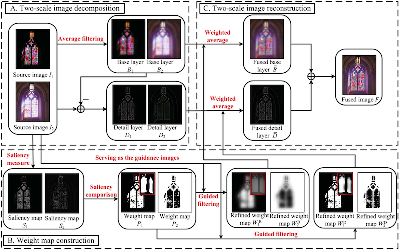
Image fusion with guided filtering
The method aims at combining several images, either in a multi-focus setting or in a multi-exposure setting.
Tip
Saliency is defined as the local average of the norm of the image Laplacian.
The images are combined through a weighted sum. The weights are determined according to the saliency map of each image, which measures the level of spatial variation at each pixel. In addition, the method aims at leveraging structural information, especially by preserving edges as much as possible thanks to guided filtering.
This method can be used indifferently for multi-focus and multi-exposure problems because in both cases, the saliency map is a relevant quantity. Indeed, in the multi-focus setting, images are salient where they are sharp, whereas in the multi-exposure setting they are salient where they are well-exposed.
Step by step
gff_focus = fusion.gff(multi_focus_sample)
Weight map
Weight maps are constructed to be \(1\) at pixel \(i\) if the image has the highest saliency (i.e. gradient norm) at pixel \(i\), and \(0\) otherwise.
plot_images(*gff_focus.weights,
            labels=['weight map 1', 'weight map 2'])
plt.show()
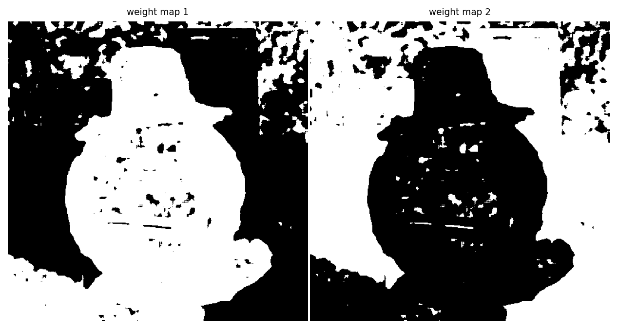
Weight maps
Base / Detail decomposition
Then, images are split into a base layer and a detail layer. Each layer will have its own weight map and be fused back in only at the very end.
base_layer, detail_layer = zip(*[gff_focus.decompose(im) for im in gff_focus.ims])
plot_images(*base_layer)
plt.show()
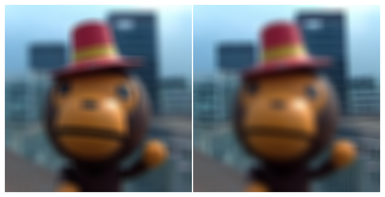
Base layers
plot_images(*detail_layer)
plt.show()
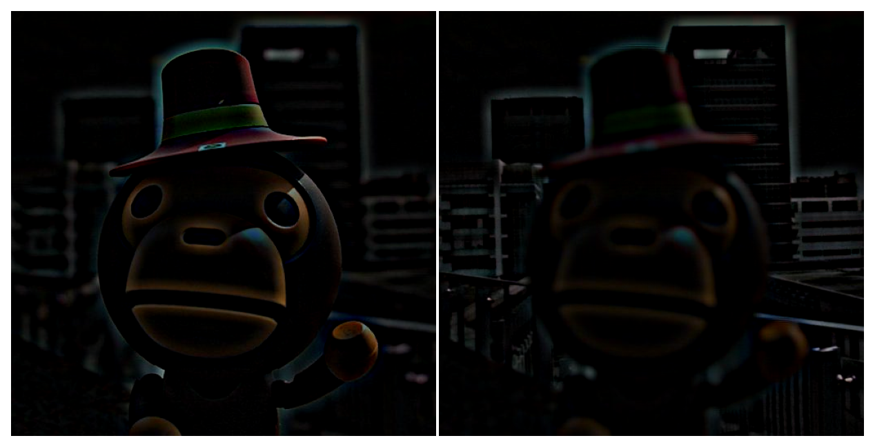
Detail layers
Refined weight map
The key idea is to use guided filtering with the original image as guidance. This mitigates noise and edge-aligns weight maps.
Different parameters (see below) are used to get distinct weight maps for the base and details layers. In general, a larger window size, and a larger regularisation \(\varepsilon\) are used for the base layer.
fused_focus = gff_focus.fusion()
plot_images(*gff_focus.refined_weights["base"])
plt.show()
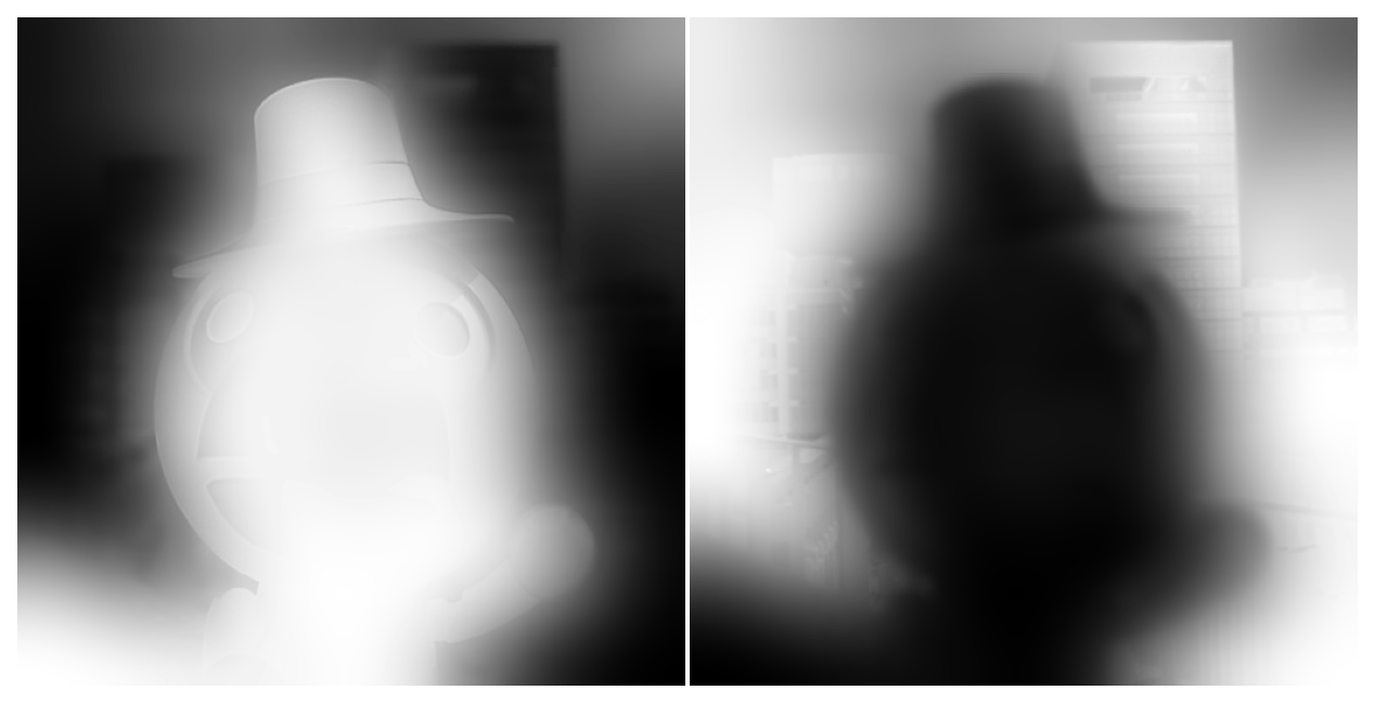
Refined weight maps (base layer)
plot_images(*gff_focus.refined_weights["detail"])
plt.show()
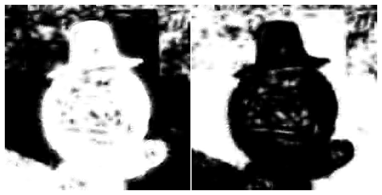
Refined weight maps (detail layer)
Fusion
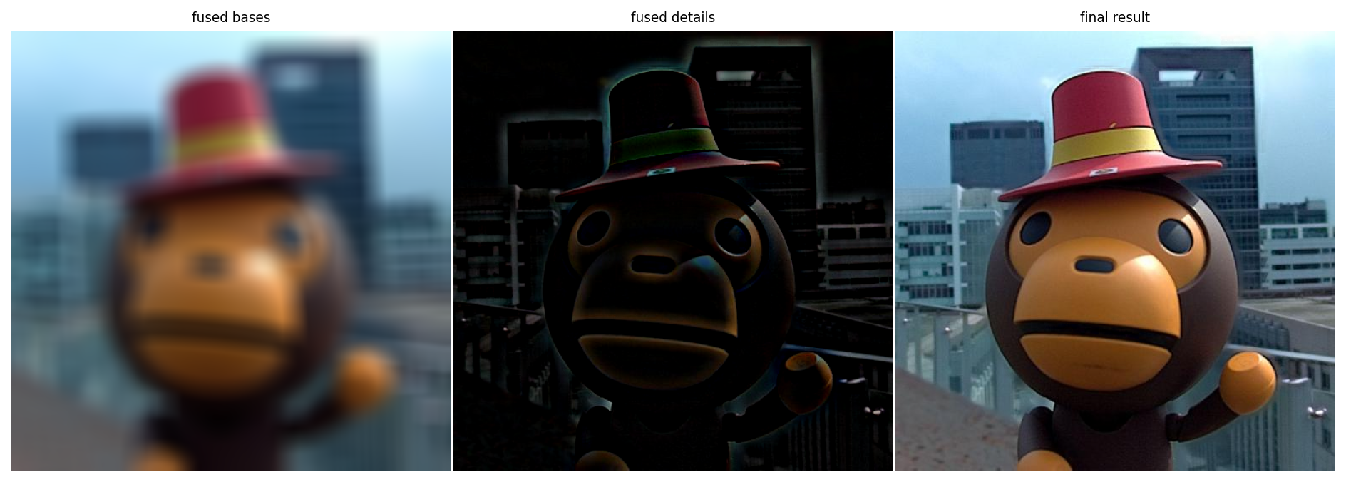
Those refined weight maps are used to fuse images in each layer base and details). Finally, the layers are added up to produce a single final image. For multi-focus, the base fusion is not that important as the base images basically look the same (a blurry version of the scene). However, for HDR, both base fusion and detail fusion must be done carefully.
plot_images(gff_focus.fused["base"], gff_focus.fused["detail"], fused_focus,
            labels=['fused bases', 'fused details', 'final result'])
plt.show()
Fusion
Examples
Because the concept of saliency discriminates both in-focus against out-of-focus, and saturated against non-saturated, the method above can actually be used both for HDR and multi-focus recomposition.
exposure_gff = fusion.gff(multi_exposure_sample)
multi_exposure_fused = exposure_gff.fusion(r1=100, r2=15)

focus_gff = fusion.gff(multi_focus_sample)
multi_focus_fused = focus_gff.fusion()

gray_gff = fusion.gff(gray_sample)
multi_gray_fused = gray_gff.fusion()
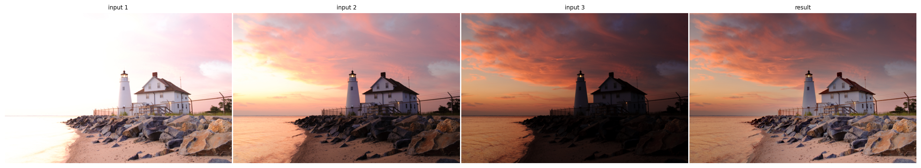
Multi exposure fusion
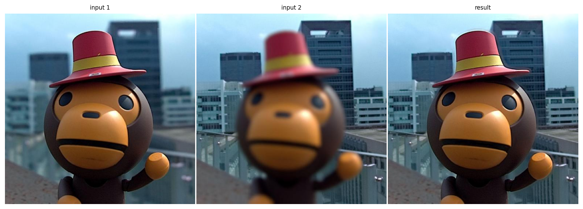
Multi focus fusion
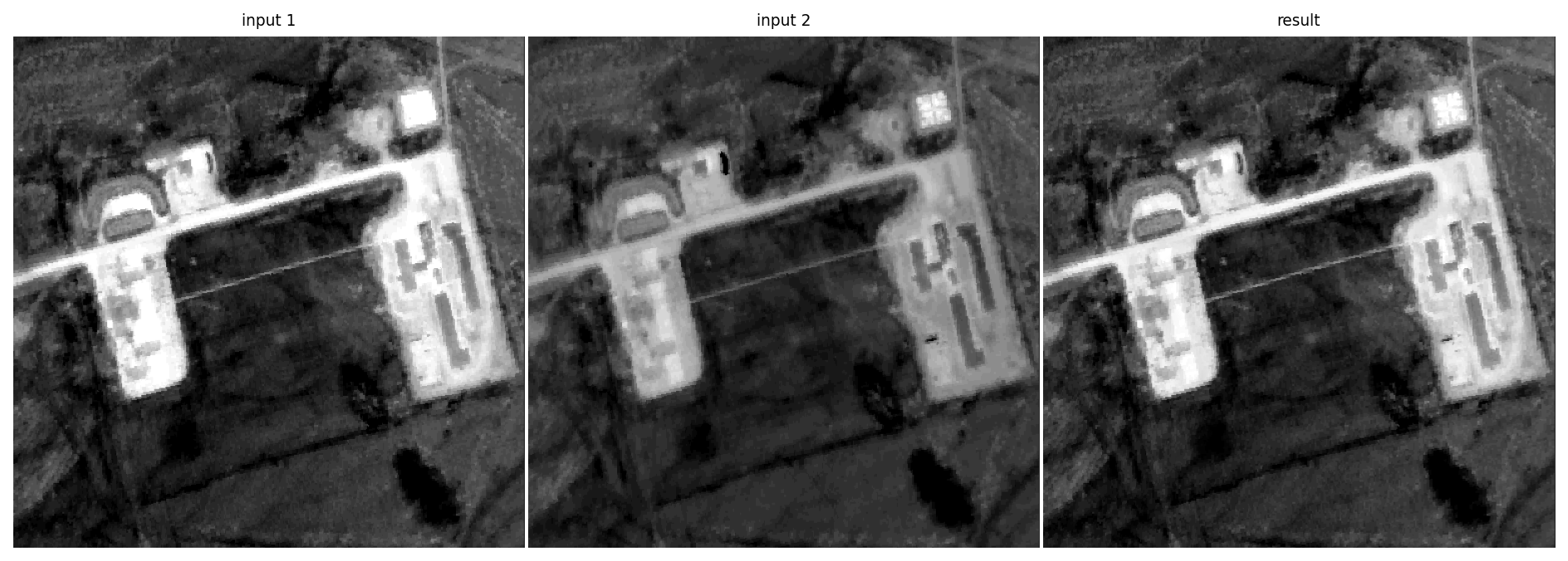
Gray fusion
Managing out-of-bounds values
The authors do not speak about how to handle out of bounds values. Out-of-bounds may appear during two steps:
When applying the guided filters, there is no guarantee that the output will stay either in the input image or guidance image bounds. It seems reasonable to clip the filtered weights between 0 and 1, otherwise we cannot normalize the weights in a meaningful way.
When recombining the base and detail layer, we can also get out-of-bounds values. Simply rescaling the output may noticeably “grayify” the image if there are values in the output too far out of bounds. We chose to also clip the image instead.