Experiments and remarks
Contents
Experiments and remarks
Our analysis mostly boils down to ablation study
Parameters and their impact
The free parameters of the fusion method are the window size and regularization for the two guided filters (for the base and detail layer, respectively). The choice of parameters can be crucial, especially for multi-exposure fusion. This is less the case for multi-focus fusion.
The article is contrasted about this issue, stating at first:
“the GFF method does not depend much on the exact parameter choice.”
However, the article ends with
“adaptively choosing the parameters of the guided filter can be further researched.”
which indicates that the question cannot be entirely dismissed, especially for multi-exposure fusion.
Input images
exposure_gff = fusion.gff(multi_exposure_sample)
multi_exposure_fused = exposure_gff.fusion(r1=100, r2=15, eps1=0.3, eps2=1e-6)
multi_exposure_fused_1 = exposure_gff.fusion(r1=3, r2=15, eps1=0.3, eps2=1e-6)
multi_exposure_fused_2 = exposure_gff.fusion(r1=1000, r2=15, eps1=0.3, eps2=1e-6)
multi_exposure_fused_3 = exposure_gff.fusion(r1=100, r2=15, eps1=1e-6, eps2=1e-6)
multi_exposure_fused_4 = exposure_gff.fusion(r1=100, r2=15, eps1=100, eps2=1e-6)
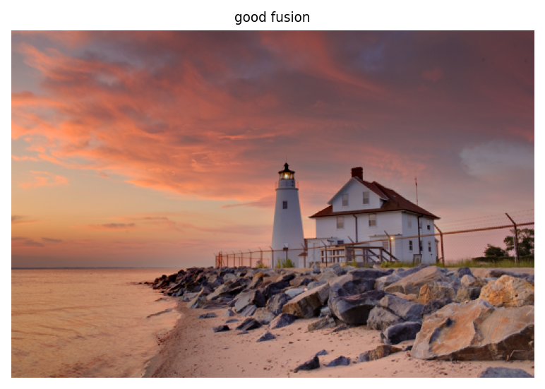
plot_images(multi_exposure_fused,
labels=['good fusion'])
plot_images(multi_exposure_fused_1, multi_exposure_fused_2,
labels=['smaller window (base layer)', 'bigger window (base layer)'])
plot_images(multi_exposure_fused_3, multi_exposure_fused_4,
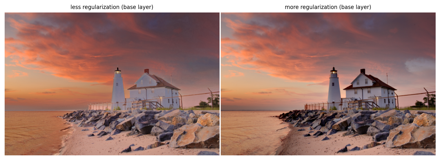
labels=['less regularization (base layer)', 'more regularization (base layer)'])
plt.show()

Influence of the base layer parameters
Influence of the base layer parameters
Influence of the base layer parameters
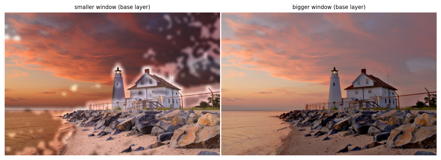
Modifying the value of either \(r\) (the window size) or \(\epsilon\) (the regulaization parameter) in the base layer parameters induces important defects.
Top row (window size \(r\)): patches appear when \(r\) is too small, and many zones are too light when \(r\) is too big (averaging on wide zones).
Bottom row (regularization parameter \(\epsilon\)): incoherent result with insufficient regularization: the house seems flat, the beach is much lighter than the sea, etc. However increasing regularization has little effect.
multi_exposure_fused_1 = exposure_gff.fusion(r1=100, r2=1, eps1=0.3, eps2=1e-6)
multi_exposure_fused_2 = exposure_gff.fusion(r1=100, r2=500, eps1=0.3, eps2=1e-6)
multi_exposure_fused_3 = exposure_gff.fusion(r1=100, r2=15, eps1=0.3, eps2=1e-10)
multi_exposure_fused_4 = exposure_gff.fusion(r1=100, r2=15, eps1=0.3, eps2=1e2)
plot_images(multi_exposure_fused,
labels=['good fusion'])
plot_images(multi_exposure_fused_1, multi_exposure_fused_2,
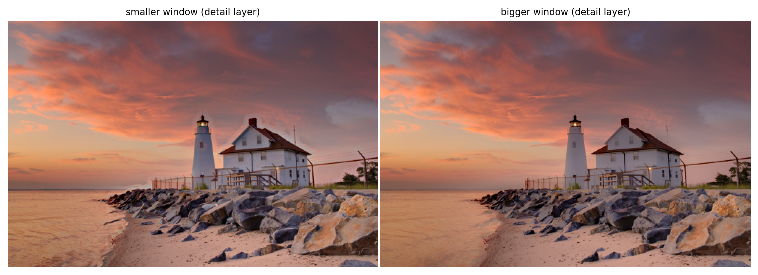
labels=['smaller window (detail layer)', 'bigger window (detail layer)'])
plot_images(multi_exposure_fused_3, multi_exposure_fused_4,
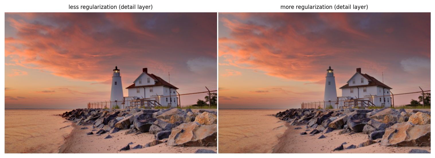
labels=['less regularization (detail layer)', 'more regularization (detail layer)'])
plt.show()
Influence of the detail layer parameters
Influence of the detail layer parameters
Influence of the detail layer parameters
Most changes are less noticeable when toying with the details layer parameters, probably because the layer is more sparse.
Top row (\(r\)) : once again, patches appear when \(r\) is too small (even though less noticeably), but more importantly details are lost when \(r\) is too big.
Bottom row (\(\epsilon\)): no noticeable changes.
Is guided filtering necessary?
The authors suggest guided filtering as a filter method which knows about the structure of the (source/guide) image, and specifically its edges. We investigated how useful this method was against:
no-filtering
a naive gaussian filter
No filtering
It is necessary to perform some kind of smoothing, in order to prevent patches to appear. This can be easily seen in the case of exposure fusion:
# no weights filtering
fused_exposure = exposure_gff.fusion(filt=lambda p, *args, **kwargs: p)
plot_images(*multi_exposure_sample)
plot_images(*exposure_gff.normalised_refined_weights["base"]) #same as detail

plot_images(fused_exposure)
No filtering
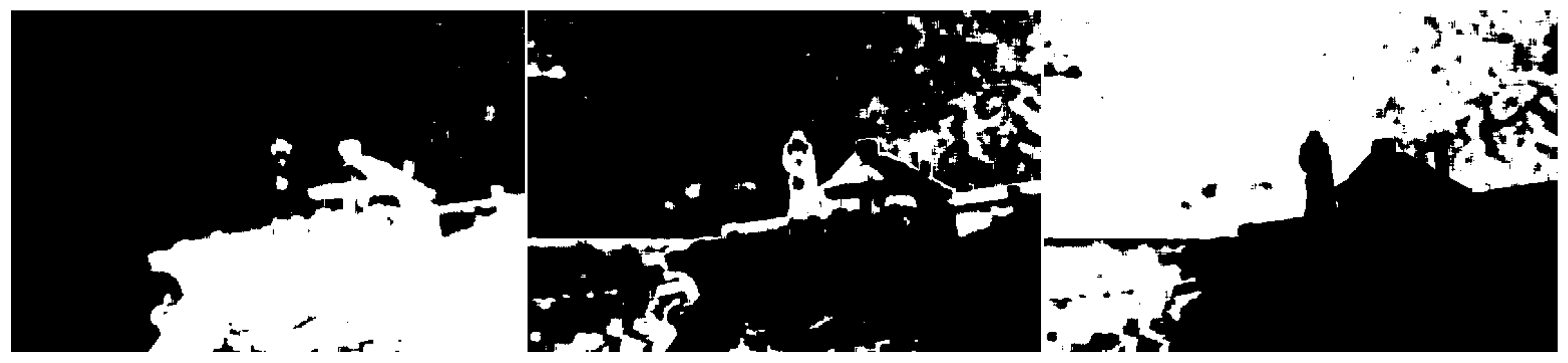
No filtering
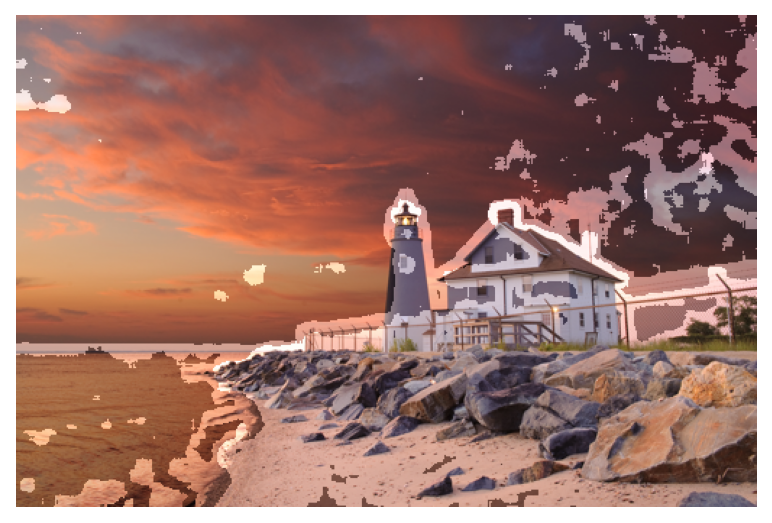
No filtering
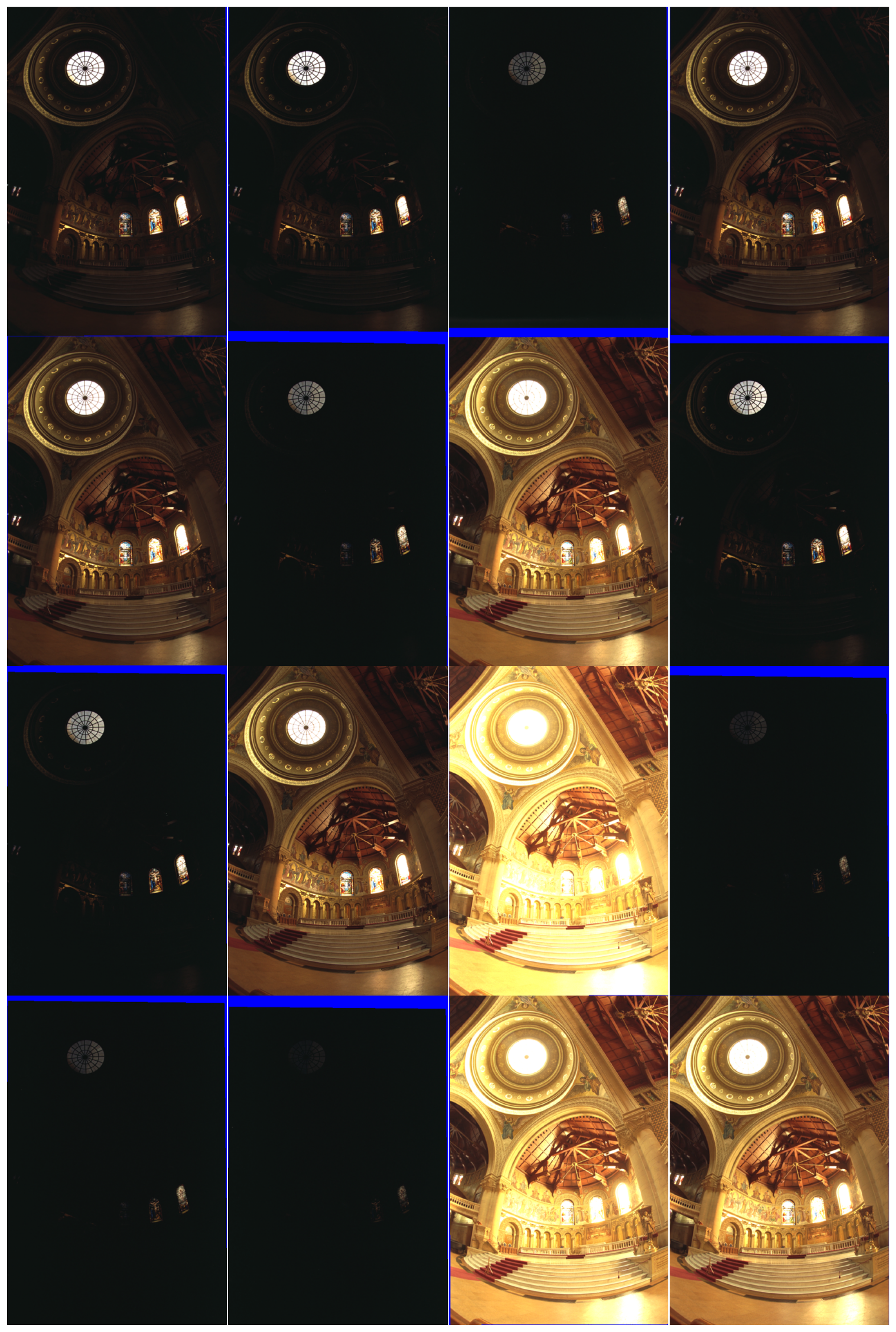
Gaussian filtering
What about using a gaussian filter instead of a guided filter that leverages the structure of a guidance image?
def gaussian_filter(p,i,r,eps):
  return gaussian(p, r)
multi_exposure_sample = multi_exposure_dataset["Memorial_Debevec97"]
exposure_gff = fusion.gff(multi_exposure_sample)
plot_images(*multi_exposure_sample, maxwidth=4)
# Guided filter with source image as guide
fused_exposure = exposure_gff.fusion(r1=20, eps1=1e-2)
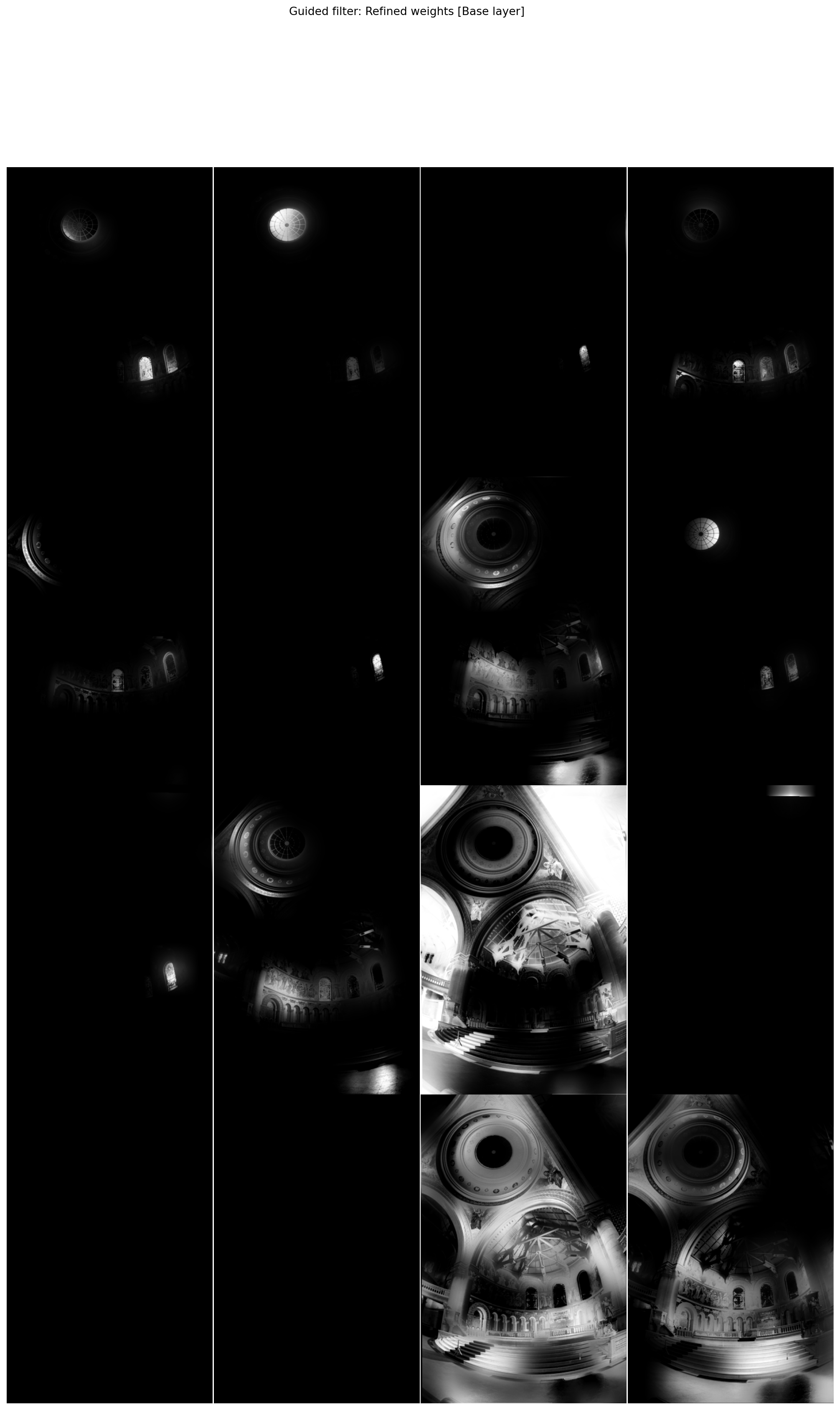
plot_images(*exposure_gff.normalised_refined_weights["base"],
title="Guided filter: Refined weights [Base layer]",
maxwidth=4)
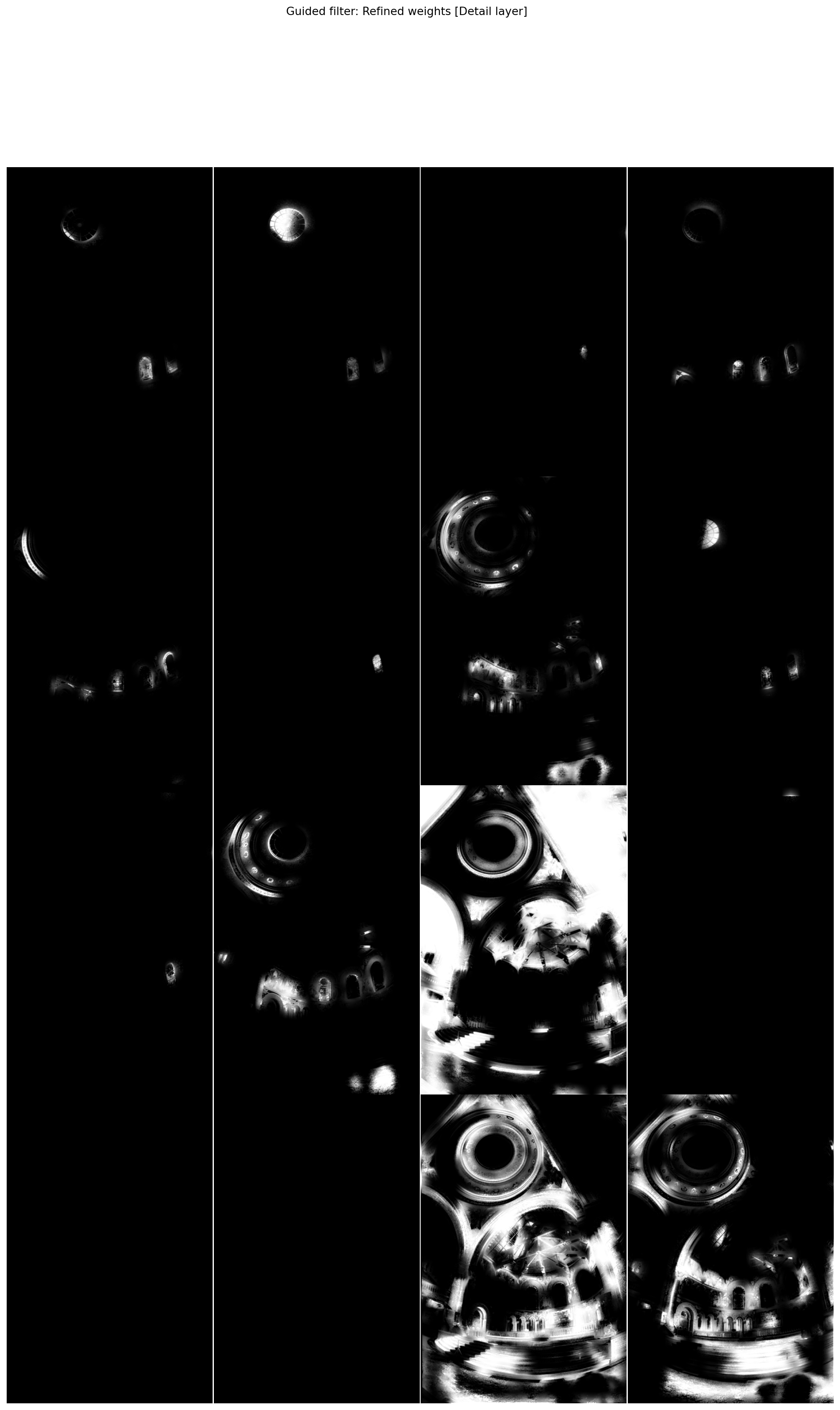
plot_images(*exposure_gff.normalised_refined_weights["detail"],
title="Guided filter: Refined weights [Detail layer]",
maxwidth=4)
plt.show()
# Gaussian filter
fused_exposure_gauss = exposure_gff.fusion(filt=gaussian_filter,
                                           r1=10)

plot_images(*exposure_gff.normalised_refined_weights["base"],
            title="Gaussian filter: Refined weights [Base layer]",
            maxwidth=4)

plot_images(*exposure_gff.normalised_refined_weights["detail"],
            title="Gaussian filter: Refined weights [Detail layer]",
            maxwidth=4)
plt.show()


plot_images(fused_exposure_gauss, fused_exposure,
            labels=['Gaussian filtering fusion', 'Guided filtering fusion'])
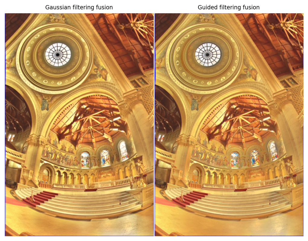
Gaussian filtering yields less satisfying results than guided filtering, especially in the most difficult zones (here around the stained glasses).
However, it is much faster, so in terms of real life applications it might be more useful.
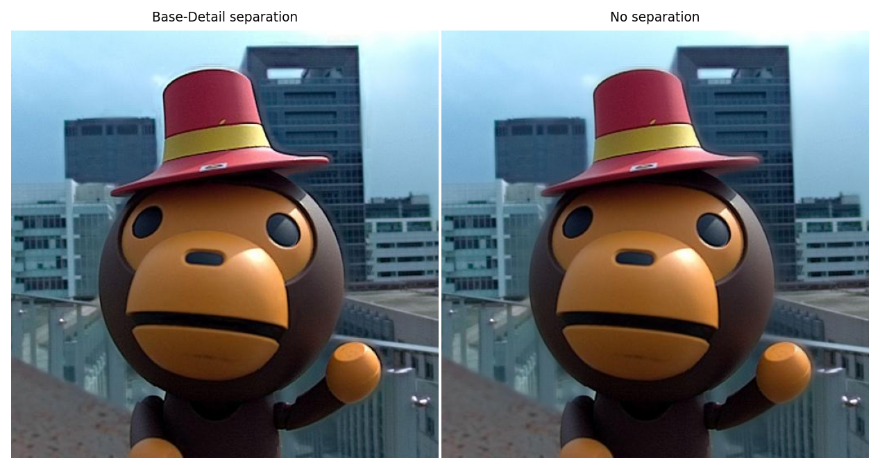
Base/detail separation
The base / detail separation is only useful to use different guidance parameter for the guided filtering. However, as shown figure 8 of the article, the dependance to those parameters seems minimal.
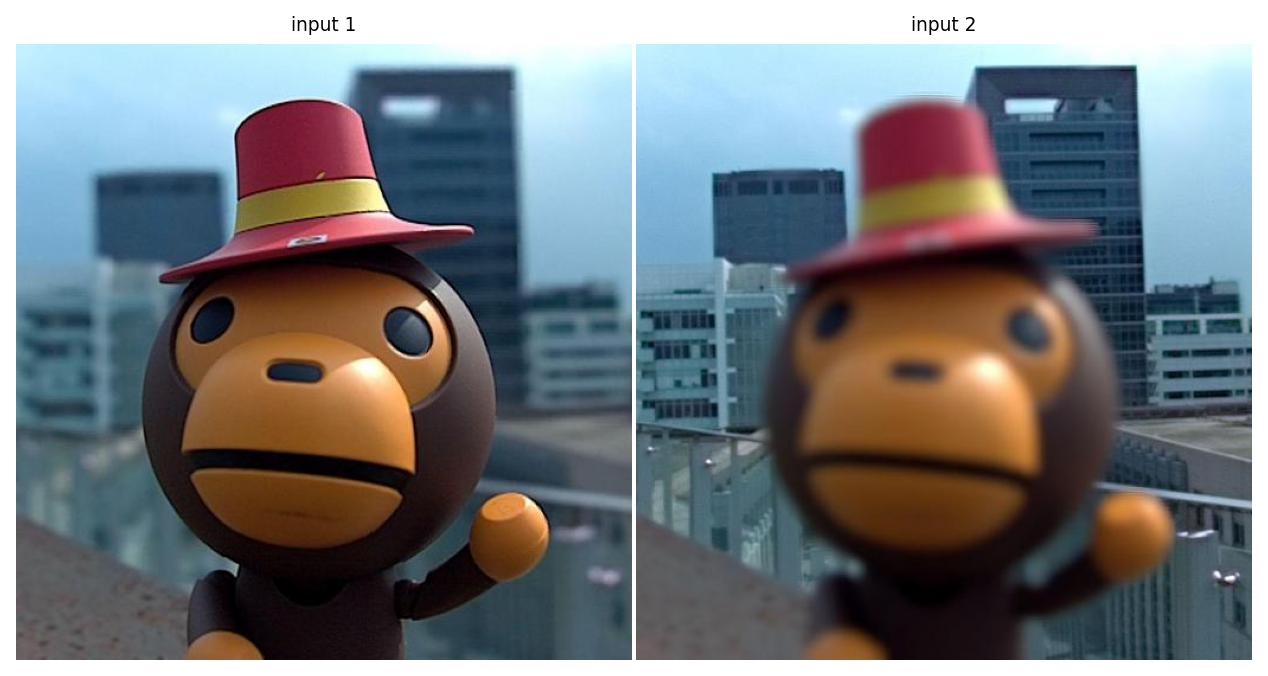
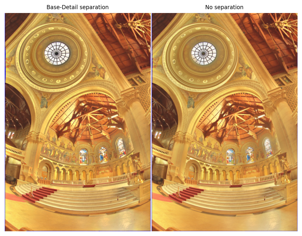
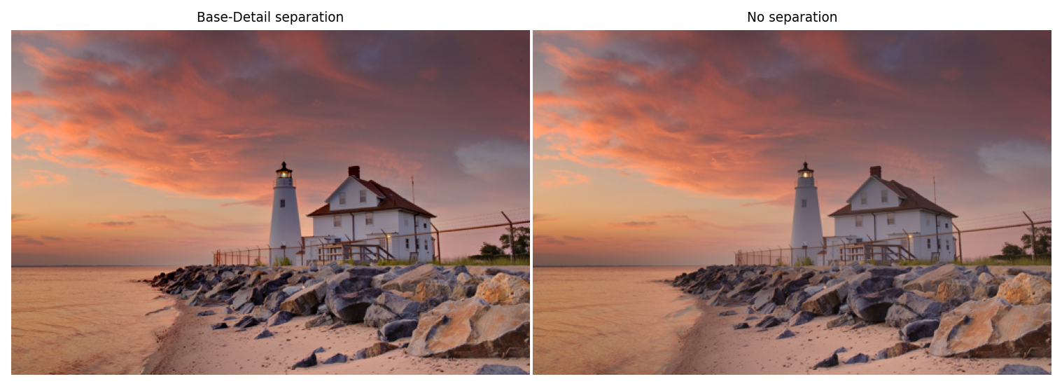
Here we show that in most cases (but not all), it seems that the base/detail separation is actually not necessary. In several examples below, the results are extremely similar (in fact indistinguishable to the naked eye) when using or not base/details separation:
multi_focus_sample = multi_focus_dataset["20"]
focus_gff = fusion.gff(multi_focus_sample)
multi_focus_fused = focus_gff.fusion()
multi_focus_fused_no_sep = focus_gff.fusion_without_separation(r=20)


plot_images(*multi_focus_sample,
            labels=['input 1', 'input 2'])


plot_images(multi_focus_fused, multi_focus_fused_no_sep,
            labels=["Base-Detail separation", "No separation"])
plt.show()
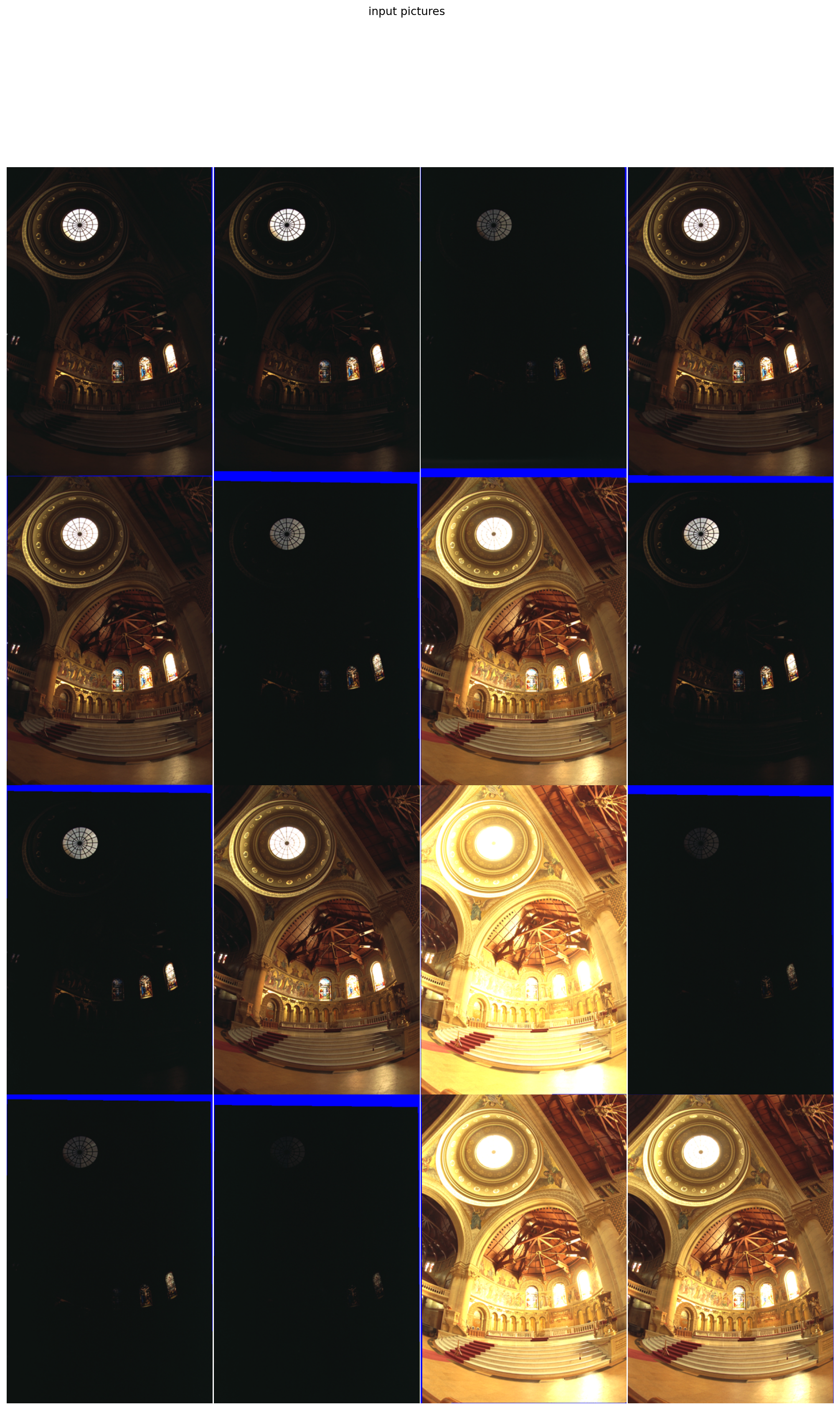
multi_exposure_sample = multi_exposure_dataset["Memorial_Debevec97"]
plot_images(*multi_exposure_sample, maxwidth=4,
            title = "input pictures")
plt.show()
exposure_gff = fusion.gff(multi_exposure_sample)

multi_exposure_fused = exposure_gff.fusion(r1=20, eps1=1e-2)
multi_exposure_fused_no_sep = exposure_gff.fusion_without_separation(r=20, eps=1e-2)

plot_images(multi_exposure_fused, multi_exposure_fused_no_sep,
            labels=["Base-Detail separation", "No separation"])
plt.show()
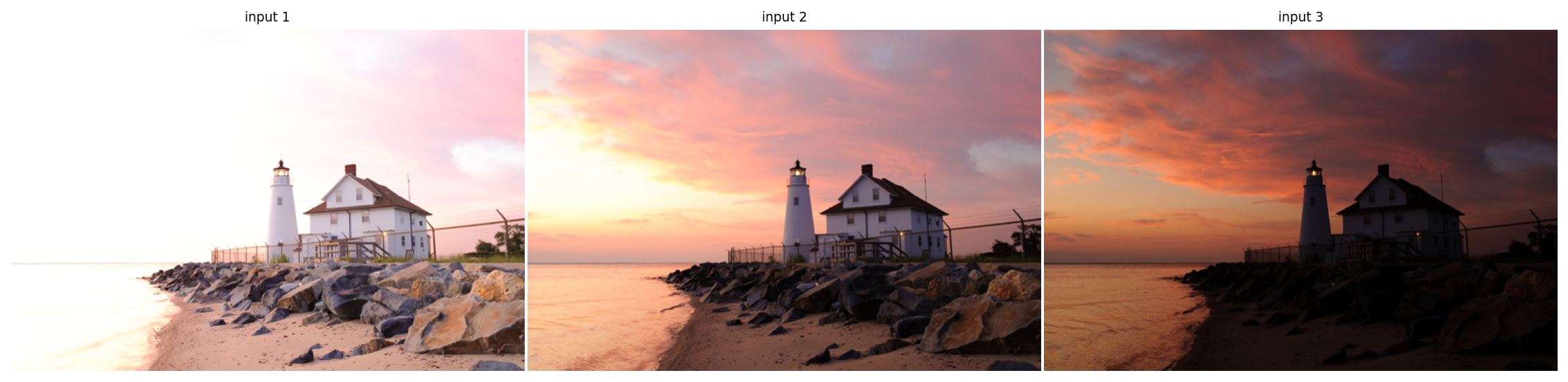
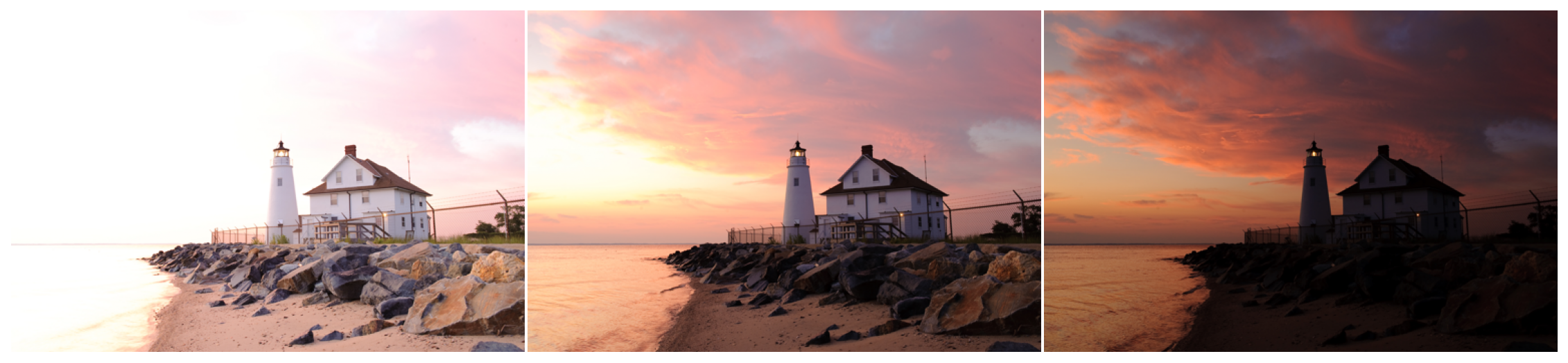
multi_exposure_sample = multi_exposure_dataset["Lighthouse_HDRsoft"]
exposure_gff = fusion.gff(multi_exposure_sample)

multi_exposure_fused = exposure_gff.fusion(r1=100, r2=15)
multi_exposure_fused_no_sep = exposure_gff.fusion_without_separation(r=100)

plot_images(*multi_exposure_sample,
            labels=["input 1", "input 2", "input 3"])


plot_images(multi_exposure_fused, multi_exposure_fused_no_sep,
            labels=["Base-Detail separation", "No separation"])
plt.show()

However, sometimes it is impossible to find a satisfying (\(r, \epsilon\)) combination. The base/details separation allows to use distinct (\(r, \epsilon\)) pairs for each layer.
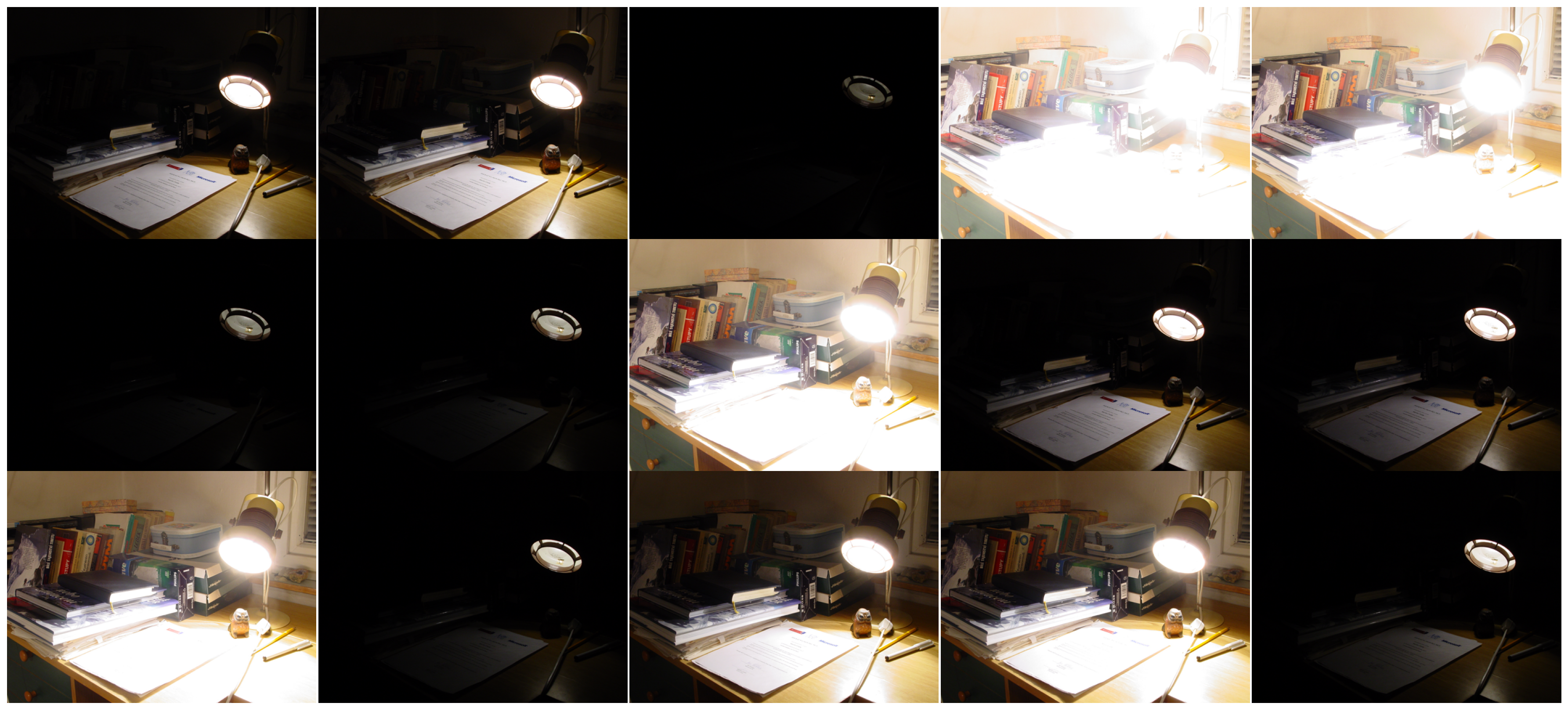
multi_exposure_sample = multi_exposure_dataset["Cadik Lamp_Martin Cadik"]
plot_images(*multi_exposure_sample)
exposure_gff = fusion.gff(multi_exposure_sample)


multi_exposure_fused = exposure_gff.fusion(r1=80, eps1=1e-1, r2=5, eps2=1e-3)
multi_exposure_fused_no_sep_1 = exposure_gff.fusion_without_separation(r=80, eps=1e-1)
multi_exposure_fused_no_sep_2 = exposure_gff.fusion_without_separation(r=20, eps=1e-1)
plot_images(multi_exposure_fused, multi_exposure_fused_no_sep_1,
            labels=["Base-Detail separation", "No separation [1]"])

plot_images(multi_exposure_fused, multi_exposure_fused_no_sep_2,
            labels=["Base-Detail separation", "No separation [2]"])
plt.show()
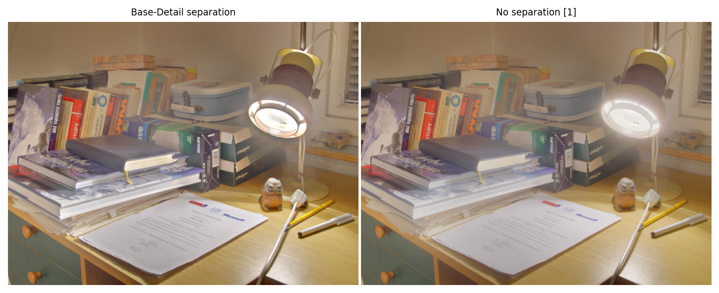
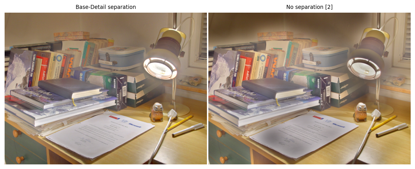
Here, without base/details separation (right side), we either have a halo around the lamp or dark patches on the sheet of paper and on the walls.
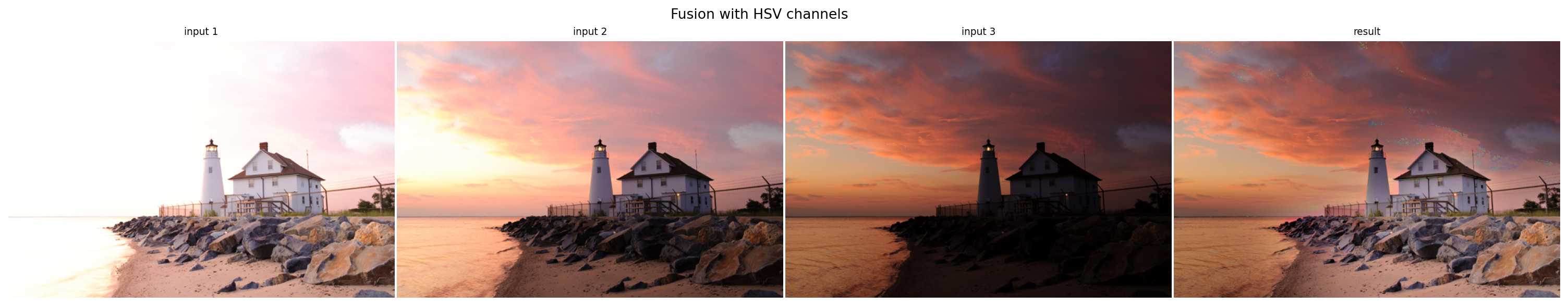
Other color spaces: HSV
The method works just as well with color spaces other than RGB, for example HSV, despite the doubtful relevance of doing linear combinations of the coefficients in the energy formula (and despite the discontinuity in the Hue channel).
from matplotlib.colors import rgb_to_hsv, hsv_to_rgb
multi_exposure_sample = multi_exposure_dataset["Lighthouse_HDRsoft"]

# data: rgb to hsv
hsv_input = [rgb_to_hsv(im) for im in multi_exposure_sample]

# gff
hsv_gff = fusion.gff(hsv_input, color='hsv')
fused_hsv = hsv_gff.fusion()

# result: hsv to rgb
result = hsv_to_rgb(fused_hsv)
plot_images(*multi_exposure_sample, result,
            labels=['input 1', 'input 2', 'input 3', 'result'],
            title="Fusion with HSV channels")
plt.show()
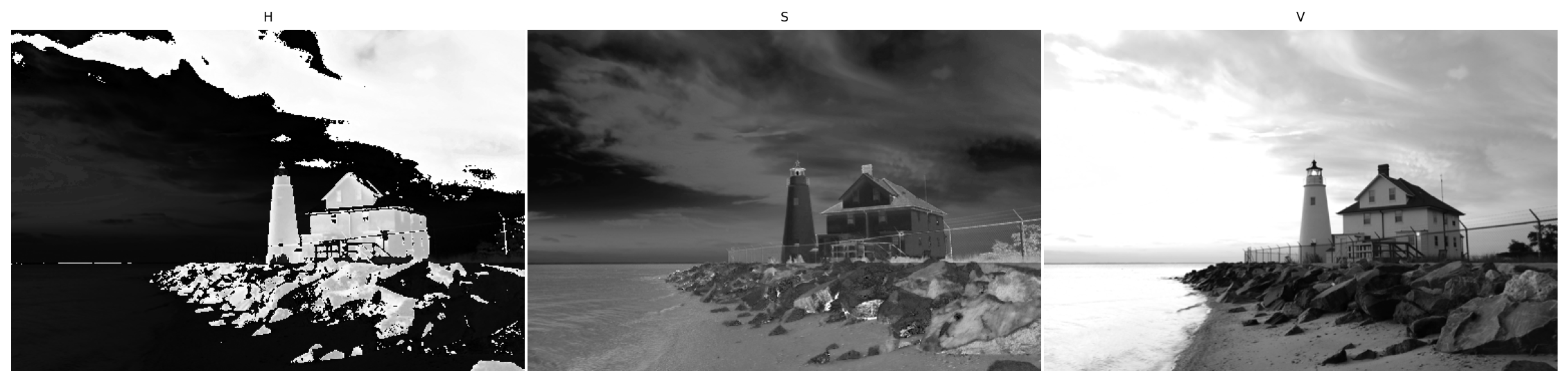
By examining the application of the guided filter, we see that sharp edges remain as long as there is the V channel in the guide. The H channel is also necessary in order to avoid color artefacts.
im_hsv = hsv_input[1]
h, s, v = im_hsv[:,:,0], im_hsv[:,:,1], im_hsv[:,:,2]

plot_images(h, s, v, labels=["H", "S", "V"])

out_v = hsv_to_rgb(filters.guided_filter(im_hsv, v, r=7, eps=1e-3))
out_h = hsv_to_rgb(filters.guided_filter(im_hsv, h, r=7, eps=1e-3))
out_full = hsv_to_rgb(filters.guided_filter(im_hsv, im_hsv, r=7, eps=1e-3))

plot_images(out_v, out_h, out_full,
            labels=['V guide only', 'H guide only', 'full guide'],
            title="Guided filtering (HSV space)")
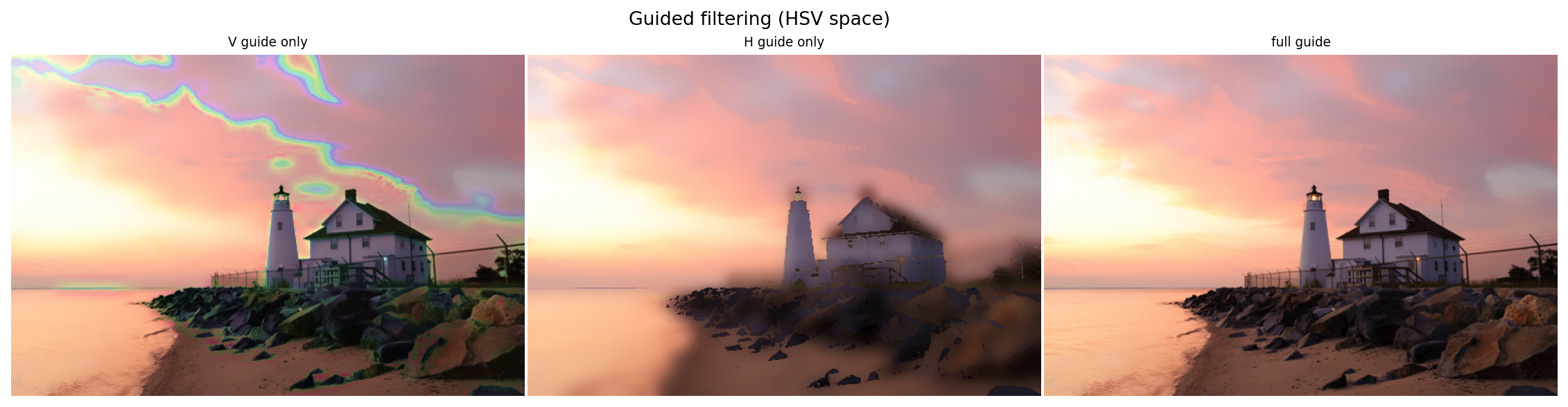
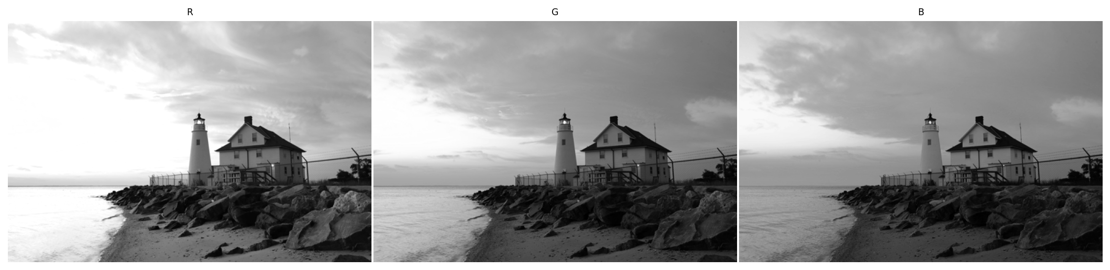
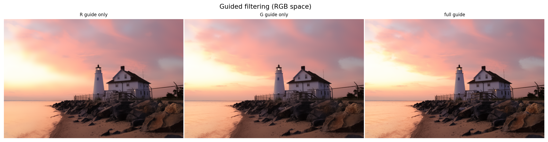
By contrast, on a standard image, all three RGB channels roughly share the same edges thus yield satisfying results as the guide.
im_rgb = multi_exposure_sample[1]
r, g, b = im_rgb[:,:,0], im_rgb[:,:,1], im_rgb[:,:,2]

plot_images(r, g, b, labels=["R", "G", "B"])


out_r = filters.guided_filter(im_rgb, r, r=7, eps=1e-3)
out_g = filters.guided_filter(im_rgb, g, r=7, eps=1e-3)

out_full = filters.guided_filter(im_rgb, im_rgb, r=7, eps=1e-3)

plot_images(out_r, out_g, out_full,
            labels=['R guide only', 'G guide only', 'full guide'],
            title="Guided filtering (RGB space)")